In the event that we have tried on occasion to paste something in a table that has been filtered, we will surely have verified that it is not as easy as it seems. When copying tables, we are likely to copy hidden rows or columns on occasion. This is something that can be misleading, especially if we use Excel to calculate sums of collected data. Other times, we simply want to copy only the visible rows and leave the hidden ones behind.
That is why we are going to see how we can copy data from a filtered dataset and how to paste it into a filtered column while omitting the cells that are hidden.
Copy visible cells in Excel
In the event that some cells, rows or columns of a spreadsheet do not appear, we have the option of copying all the cells or only those that are visible. By default, the Microsoft spreadsheet program copy hidden or filtered cells, in addition to those that are visible. In the event that we do not want it, we must follow the steps detailed below to copy only the visible cells.
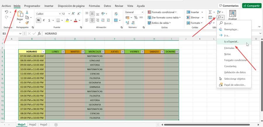
To do this we must select the cells we want to copy. Then we go to the “Start” tab. Here we click on “Search and select” that we find on the right side represented by the icon of a magnifying glass. This will display a menu where we will select the option to “Go to Special”.
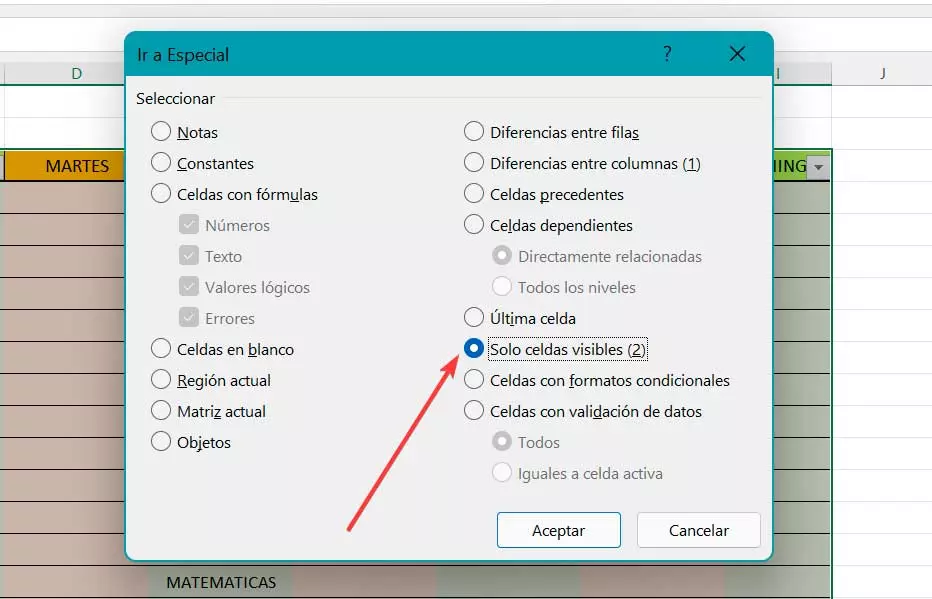
This will make a new pop-up window appear where we can choose between the multiple options that it allows us: cells with comments, constants, formulas, blank spaces, cells with data validation, etc. Here what interests us is the option of “Only visible cells”so we click on it to select and click on “OK”.
Next, with the cells selected we press for which we can use the keyboard shortcut Ctrl + C, or right-click and select Copy. We can also click directly on the Copy icon (two-page icon) that we find within the Clipboard section on the Home tab.
Now we only have to move to the box where we want to paste the cells that we have copied and use the Paste action. To do this, we can use the keyboard shortcut Ctrl + Vright-click and select Paste, or click the Paste option found inside the clipboard on the Home tab.
Copy from a filtered column without the hidden cells
Let’s take as an example that we have a table with a schedule, with the columns that are the days of the week and the rows that are the hours. From it we want to copy all the rows for WEDNESDAY that include MATH. For this we must apply a filter.
First we will select the entire table and click on the Data tab. Here we select the button “Filter” that we find within the “Sort and filter” group.
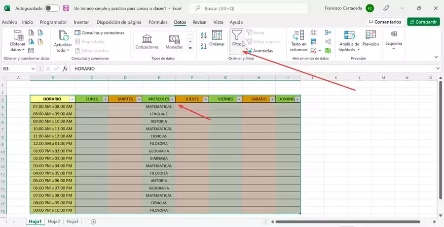
This will make small arrows appear in each cell of the header row, which will help us to filter, since it will only be necessary click any arrow to choose a filter for the corresponding column. In this case, as we want to filter the MATHEMATICS rows within the WEDNESDAY section, we select the arrow in this heading.
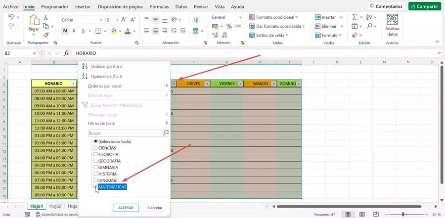
Now a pop-up appears where we uncheck the box “Select everything” and we left marked only the one of MATHEMATICS. Finally, we click on “Accept” and we will only see the rows in which MATHEMATICS appears within the schedule.
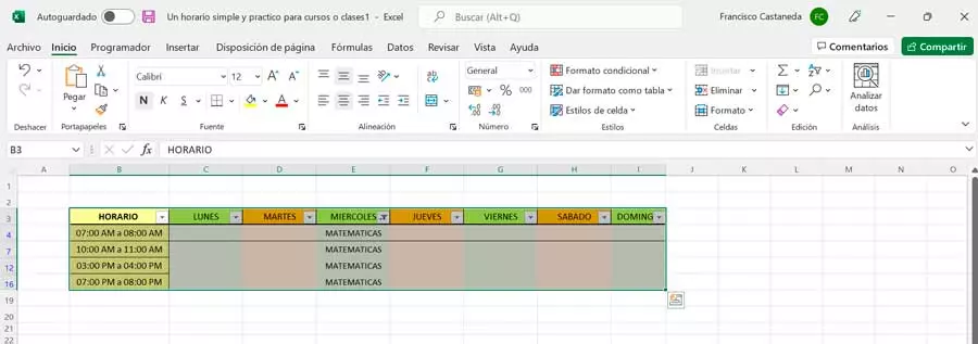
Next, copying from a filtered table is easier, because when we copy from a filtered column or table, Excel automatically copies only the visible rows. Therefore, we only have to select the visible rows that we want to copy and press any of the Copy methods, such as Ctrl + C. We select the first cell where we want to paste the copied cells and press any of the Paste methods, such as Ctrl + V, and the cells will be pasted.
Also in Google Sheets
The Google Spreadsheets application is an Excel-like program with which it shares many features and is web-based. From Sheets we can also copy and paste only the cells that are visible. To do this we must access its website and open the project we are working on and want to perform this function.
To do this, we hold down the Ctrl key and click on all the visible cells that we want to copy. Once all are selected, we copy them using the keyboard shortcut “Ctrl + C” or by using the right click. Later we paste the rows in a different location or in another file.
Copy a filtered column
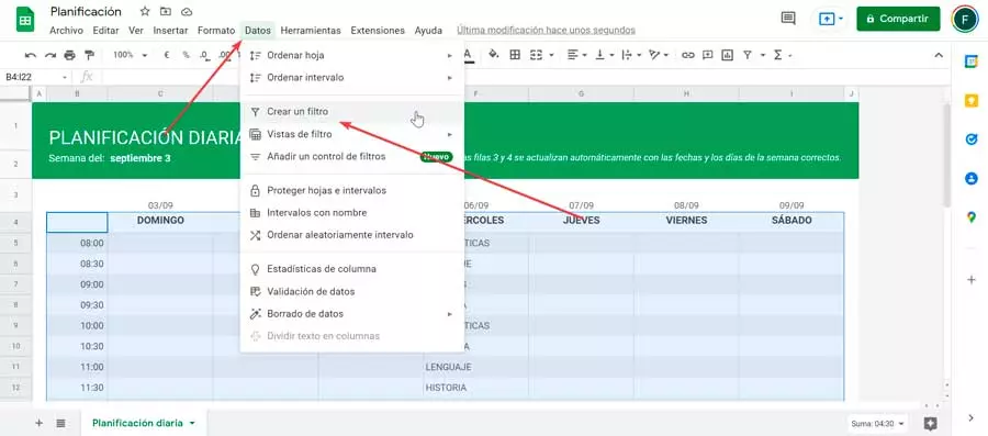
In the event that we want to copy a filtered column without the hidden cells appearing, we must do the following steps. Suppose we have a table with a schedule and we want to copy all the rows from WEDNESDAY that include MATH. For this we must apply a filter. First we will select the entire table and click on the “Data” tab. Here a menu will open where we click on “Create a filter”.
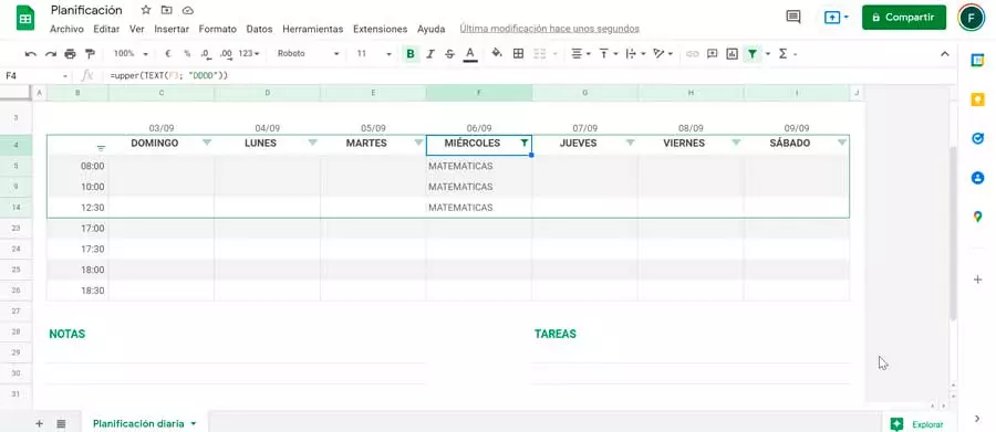
This will make some arrows appear in the header of each column that will help us to create the filter. We click on the desired arrow, in this case WEDNESDAY. We scroll to the bottom and uncheck all the options except MATH and click “OK”. This will cause that we only see in the rows that the MATHEMATICS appear within the WEDNESDAY schedule.

Like we can buy, by doing this we have filtered out all the cells we needed in a column, so now we can easily copy and paste the visible cells.
Now we only have to select the visible rows that we want to copy and use the shortcut «Ctrl + C». Subsequently, we select the first cell where we want to paste the copied cells and press the Paste option with the shortcut «Ctrl + V», and the cells will be pasted.