Microsoft’s popular spreadsheet-focused program, Excel, offers us a huge number of formulas or functions to get the most out of our projects. We can find these divided into several categories in order to be able to locate the one that most interests us in each case in a faster way. If we focus on statistical work, one of the most used formulas is that of variance.
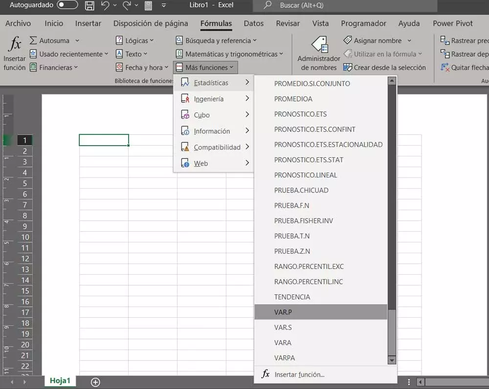
As it could not be otherwise, when carrying out this type of calculations in particular, the powerful program that is part of the suite Office Will help us. In fact, we should know that when starting the main interface of the spreadsheet application we find a menu called precisely Formulas. In it, a series of categories are distributed that implement the functions related to it in order to facilitate the location of one in particular.
Well, at this point it is interesting to know that once the categories are called Statistics. As you can imagine, here we find a good number of elements of this type for those who need to perform statistical calculations in Excel.
What is variance in statistics
Here we are going to focus, as we mentioned before, on the variance function that we can use in the Microsoft program, Excel. But first of all we should be clear about what this is really about. It is worth mentioning that the variance in statistics refers to the variability of the data that we take as a reference point in the spreadsheet.
You have to know that statistical analysis is important measure the degree of dispersion of these data. By this we mean that the number of values that is uniform or not with respect to their average must be known. This is something that we can find out precisely with the variance function in Excel, as we will see below. To do this, the first thing we do is enter the statistical data with which we are going to work here in the table.
How to Calculate Variance in Excel
Once we have them on the screen, we go to another empty cell, which is where we are going to visualize the variance that interests us. Initially, the formula that we are going to use in this case is =VAR.P. Here the variance is calculated based on all the exposed data. The format to use here is as follows:
=VAR.P (A1:A6)
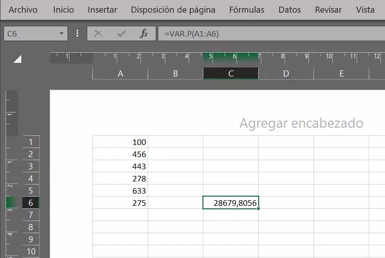
As you can imagine, the two values in parentheses in Excel refer to the range of data on which we are going to work in our document. In the example above it refers to the data in the column between cells A1 and A6. On the other hand, in the event that statistically we do not have all the databut from a sample, it is recommended to use the formula =VAR.S. This allows obtaining a more approximate result, although the format used here is the same as the one exposed.
Similarly, if we only have a sample with which to perform the statistical calculation, but also we want to include logical valueswe use the formula =VARA. To finish, we will tell you that we do have all the values, but we are also going to include the logical ones, here we opt for the option =VARPA.
Say that the format in all cases is the same as the one exposed in the previous example. All this will help us when calculating the variance in excel depending on the data we have.