
Work with large volumes of data is one of many Excel utilities. The book format combines the two dimensions of a sheet, with the third dimension that provides the possibility of using several in the same document and performing operations with the data on them. Not in vain, the calculation capacity provided by the first applications of this type, back in the eighties, were the main direct route of entry of computers in offices.
From the days of VisiCalc and SuperCalc, or the former Lotus 1-2-3 reference, to Microsoft Excel, these applications have undergone a sensational evolution both in functions and in the volume of data that they are capable of generating. I still remember, for example, the limitation of 256 columns in the first versions of Excel I worked with, a few years ago. Now, for the vast majority of needs, the power of spreadsheets is more than enough.
Now, although Excel is perfectly capable of managing such volumes of data, there are tasks that are still just as complex, and as a general rule are those that fall on the user. And it is that reviewing data, something that sometimes can only be done manually, can be complex and tedious, and leave plenty of room for errors. Obviously we can use automatic sorting systems, but in tables with several columns, we may prefer to keep the original order and visually identify the values we are looking for in each of the columns.
In these circumstances, it would be most practical to have some function that would provide us with some visual element that would help us identify the values we are looking for, right? Well, the truth is that this function exists, it is called Conditional Formatting and, as its name suggests, it applies one or another format to the cells, depending on their content with respect to the rest of the range to which said format is applied.
Excel conditional formatting, step by step
For better understanding, let’s see it with an example. Imagine that you have a list with the sales of a year, per quarter of a long list of commercial agents. And on the right, the accumulated total for the year of each one of them. And what you want, at a glance, is to identify the sellers who have sold the most in each quarter and, of course, also those who have achieved a greater turnover in the year’s totals. The sheet could be something like this:
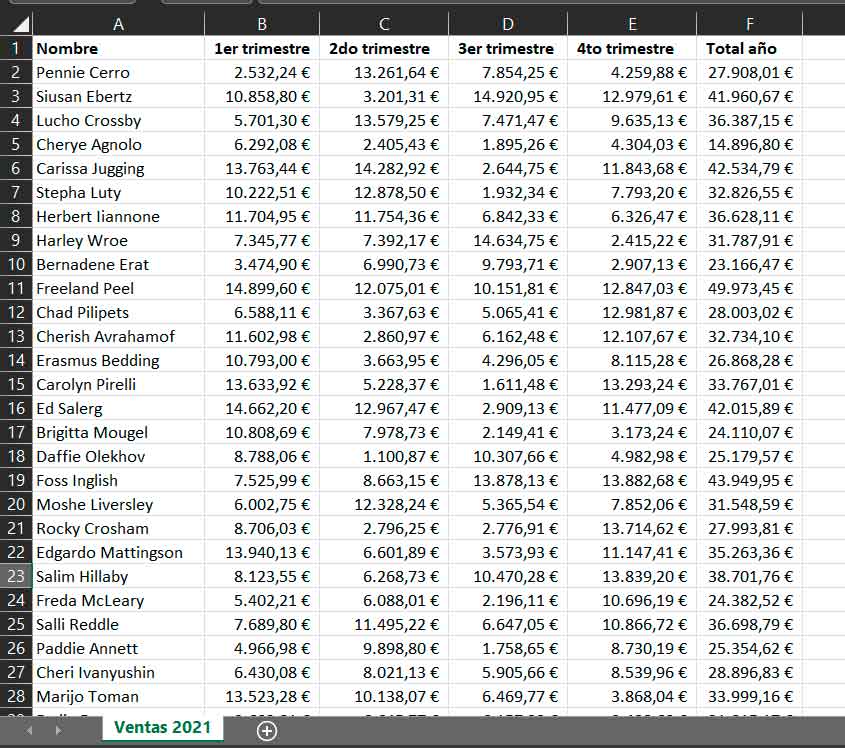
With only the 28 rows shown in the image, it already seems like a bit of a tedious task, but imagine that the list is still at the bottom… which is the case. Identifying the highest (or lowest) numbers in each column can be tedious. However, with Excel’s conditional formatting, you’ll be able to identify them in no time, and with no margin for error.
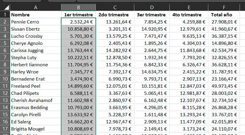
The first thing you need to do is select the cells with values from the first column. It’s important that you don’t choose every cell in every column, since you only want to compare each salesperson’s values for that quarter:
Once all the values are selected, make sure you have the Home tab selected on the top ribbon and locate the Conditional Format button. Then click on it, so that the menu is displayed

As you can see, this tool offers a huge set of options, along with the flexibility of being able to create your own conditional formats. However, for this first contact with the function, we will stick with the predesigned formats, which are perfectly useful for what we want.
The formats grouped in Rules for higher or lower values (the second menu entry) will allow you, as their name suggests, to highlight the highest or lowest values. You can do it by choosing a fixed number of them or a percentage. As you can see, the four entries in this regard offer you “10” and “10%”. If it fits what you are looking for, perfect, choose the one you prefer. But if you want to adjust the number (or the percentage) click on “More rules” and use the window that will be displayed for said customization

Once you have selected and confirmed the conditional formatting you want to apply, the number of values you have chosen will be highlighted in the column
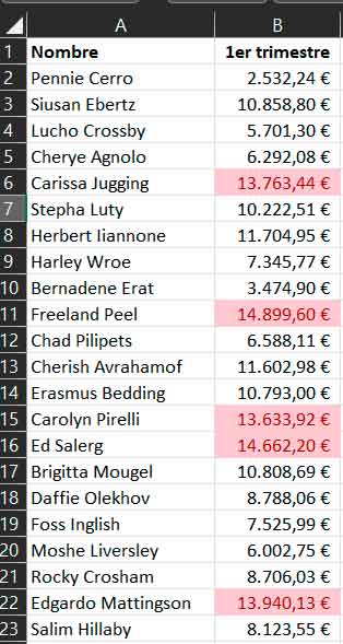
Bear in mind, and this is very important, that conditional formatting is dynamic, so if you modify the value of the cells, all the corresponding changes will automatically take place.
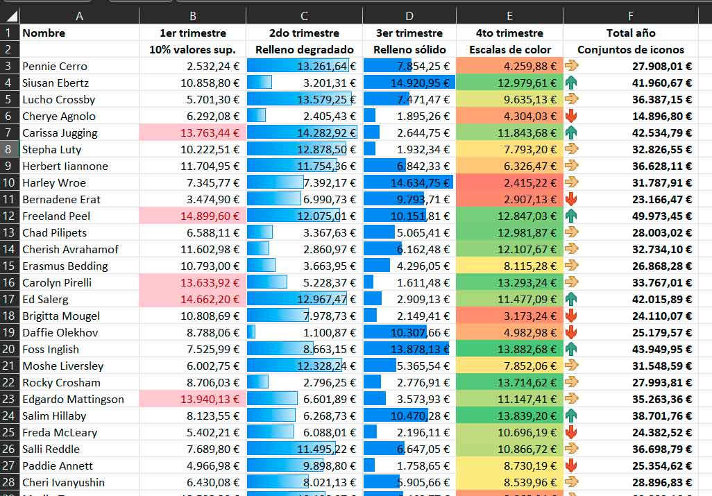
As you may have already seen when exploring the function, conditional formatting offers you multiple styles, so my recommendation is that you explore them, until you find the one that best suits what you are looking for. In the following image, you can see five different conditional formatting styles, among those that you can find in Excel. In row 2, under the quarter and above the data, you can see the name of each of them. And, as you can see, there are the most varied options
If you like Excel tricks, remember that we also recommend these three that will make your life easier, and that we have also told you how to calculate rules of three direct in inverse, and also how to calculate different types of percentages.
Learn more about Excel: Microsoft