When we create a document, the first thing we must do is create a structure so that it is easy to read and all the information is perfectly organized and that, at a glance, we can see all the content it includes. In Word we can use the Styles function that allows us to establish a different format for each of the text sections. In Excel, the function that we must use, in combination with Styles to format tables is to combine cells.
When creating a table, it must have the corresponding title that allows us to identify what data is displayed. This title should be in the upper center of the table, implying that all the data related to the title is found in that table. The method that many users use to write the title is to find the most central cell of all and write the text changing the size and font, offering a very poor final result aesthetically and functionally speaking. The combine cells function, as we can well deduce from the name, allows us to merge multiple cells into one both vertically and horizontally.
How to merge cells in Excel
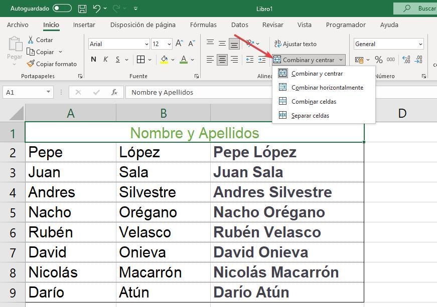
The function to merge cells in Excel is available on the Home ribbon through the Merge and Center button. But, if we click on the inverted triangle located just to the right of the button, a drop-down is shown with all options available: Merge and Center (the default and most used function), Merge Horizontally, Merge Cells, and Split Cells. Each of these functions offers us different results and that we explain below.
- Merge and center. This function combines all the selected cells into one, occupying the same size as the cells used and centering the text inside it. We can use this function both vertically and horizontally without any limit.
- merge horizontally. The Combine Horizontally function allows us to combine cells horizontally. In this way, we can combine multiple rows of data independently.
- merge cells. By clicking on this function, Excel will combine all the selected cells without aligning the text to the center. The reason the function’s default option isn’t there is because aesthetically, if we align the text displayed in the merged cells, the result is much more visually appealing.
- split cells. This is the function that we must use when we want to separate cells that have previously been combined. To use it, we just have to place the mouse on the result of the cell combination and press the Separate cells button.
Show data from two cells in one
The combine cells function is not useful if what we want is to join the data from two or more cells that are already written in a single cell, since, when combining the cells, the text of one of them disappears. The solution to this problem is as simple as applying a simple formula and hiding the columns from which the data is being extracted.
Using &
The formula that we must use to combine the data from two columns in a third column is =A2&» «&B2 taking into account that the data is found both in cell A2, which would correspond to the first name, and in cell B2, where the first surname would be found.

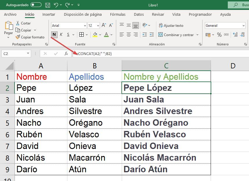
With the Concat function
Another option is to use the Concat function, a function that allows us to join several cell values into one. Continuing with the same example, if we want column C to display the first and last name of columns A and B separated by a space, we must use the formula =CONCAT(A2;» «;B2) in each of the cells in column C.
If we have any problems when applying the formula, we can use the Excel formula wizard that we can access by clicking on the fx button located just to the left of where we entered the formula we want to use and follow the instructions it indicates.